Gasoline Price Forecast Validation
Random Forest missed the July 2024 EIA value by only $0.0089 per gallon.
SARIMA came within about $0.028 per gallon of the actual May 2024 EIA value.
Lowest total error across the later April 2024 to March 2026 validation window.
This project started as a research paper focused on extracting insight from U.S. gasoline prices: how they move over time, how strongly fuel categories correlate, and how much of that behavior can be explained by trend versus outside economic shocks. From there, the analysis expanded into predictive modeling, where I built machine learning and time-series forecasting approaches using data available through roughly March 15, 2024 to test whether future price movement could be estimated from the historical series.
The validation setup is what makes the result credible. The later April 2024 to March 2026 EIA data was used as a post-training validation window to check those forward forecasts against future published values, not to rerun the same 2024 workflow on the 2026 dataset and call that validation. Within that setup, Random Forest produced the closest single 2024 hit, while SARIMA delivered the strongest overall accuracy across the broader post-training window.
I trained the forecasts on data available in March 2024, then later checked them against the real EIA prices published from April 2024 through March 2026, with the best model landing within 1 cent and the second-best within 3 cents.
Technologies Used
Capstone Focus
The paper framed gasoline as a high-impact economic variable shaped by supply, demand, policy, and global events. The central question was whether time itself could function as a statistically meaningful predictor of U.S. gasoline price movement while also helping explain longer trend behavior and seasonality.
The written analysis used inferential analysis, predictive analytics, and time series modeling on monthly EIA gasoline data. The paper also connected the observed volatility to major external shocks, especially the 2008 financial crisis and the 2022 post-pandemic price spike.
Paper Findings
The capstone concluded that time was a significant predictor, but not a complete explanation. The different gasoline product types moved together closely, indicating strong correlation across fuel categories, while the regression analysis showed that outside events still played a major role in price behavior.
2024 Forecast Check
The April to July 2024 window is where the forecast behavior becomes easy to read: April stayed close, May and June widened during a sharper price move, and July produced the standout near-exact Random Forest hit.
Key Takeaways
Closest 2024 forecast: less than 1 cent per gallon from the actual July 2024 value.
Closest 2024 forecast: about 3 cents per gallon from the actual May 2024 value.
Closest 2024 forecast: about 6 cents per gallon from the actual July 2024 value.
April to July 2024 Validation Table
| Month | Actual | Random Forest | SARIMA | Linear Regression |
|---|---|---|---|---|
| April 2024 | $3.611 | $3.596 | $3.473 | $3.527 |
| May 2024 | $3.603 | $3.726 | $3.575 | $3.533 |
| June 2024 | $3.455 | $3.708 | $3.632 | $3.540 |
| July 2024 | $3.484 | $3.493 | $3.588 | $3.547 |
This is the direct post-training check: forecasts generated from data ending March 15, 2024 compared against later published EIA prices. Across the longer April 2024 to March 2026 horizon, SARIMA delivered the lowest aggregate error, while Random Forest produced the single closest short-term hit.
Model Visuals
The original analysis produced several charts that make the forecasting logic easier to read. Taken together, they show the long-run structure of the gasoline series, the strength and limits of the linear fit, the shared movement across fuel categories, and the seasonal behavior that makes SARIMA useful in this problem.
Retail Gasoline Prices Over Time
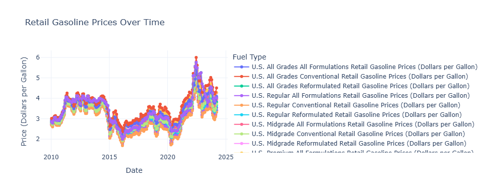
This multi-series view establishes the core problem: fuel prices move through long trend cycles, sharp shocks, and overlapping product behavior. It also makes clear why a forecasting approach has to account for both trend and volatility rather than treating the data as a simple straight-line series.
Actual vs Predicted Prices
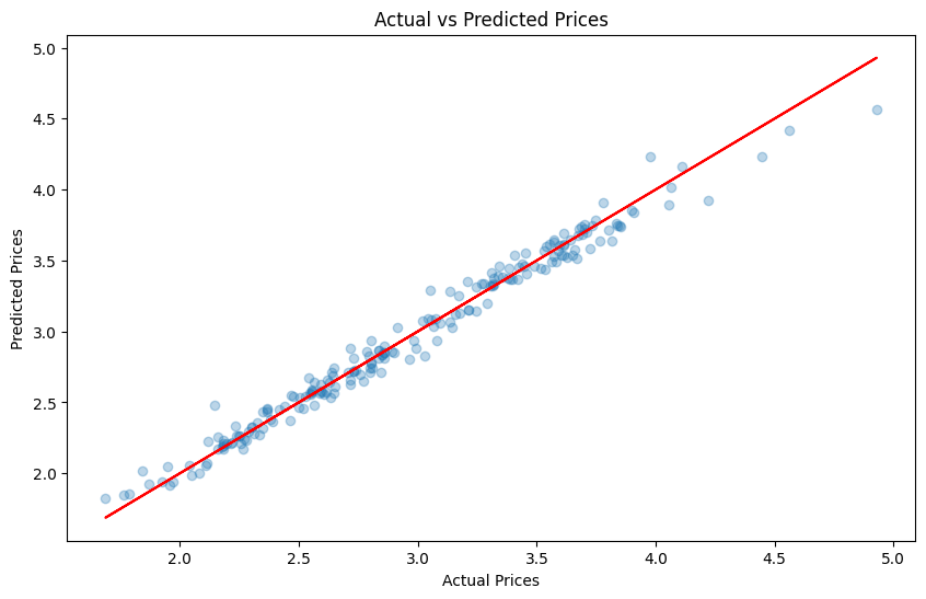
This scatter plot shows that the fitted model tracks the historical relationship reasonably well through the observed range. Points stay close to the reference line overall, but the later validation work on this page still matters because a good in-sample fit does not guarantee the strongest forward accuracy.
Time-Series Decomposition
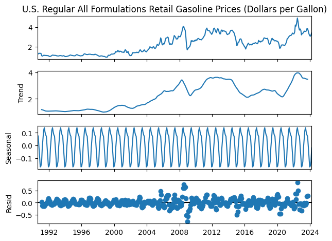
The decomposition breaks the regular gasoline series into observed behavior, underlying trend, seasonal structure, and residual noise. This is one of the clearest visual reasons SARIMA belongs in the modeling mix: the data contains recurring seasonal shape alongside longer-term price movement.
Fuel Price Correlation Matrix
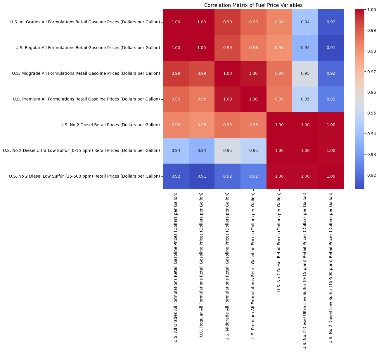
The heatmap shows how tightly the fuel categories move together. That strong shared structure supports the paper's conclusion that gasoline products are highly correlated, while also underscoring that outside economic shocks still push the whole system up or down together.
Where The Forecasts Were Generated
The later validation work traces back to specific numbered notebook cells inside the original March 2024 artifact. Those cells generated the forward-looking outputs that were later checked against the published EIA values.
Random Forest Forecast Cells
The clearest short-horizon forecast appears in In [43], where the notebook
predicts the next three months, builds prediction_dates, and stores
predicted_prices.
That same model family continues into the later forecast and plotting cells, but
In [43] is the easiest place to navigate when tracing the original
Random Forest-style forward predictions.
SARIMA Forecast Cell
The SARIMA forecast is generated in In [74], where the notebook fits the
SARIMAX(...) model and calls results.get_forecast(steps=12).
That cell produced the later twelve-month SARIMA path that was compared against the published post-March-2024 EIA values.
Linear Regression Forecast Context
The numbered linear regression implementation appears in In [71], where the
notebook converts dates to Date_ordinal, fits LinearRegression(),
and prepares the regression trend output.
That time-based regression path is the basis for the validation comparison shown here alongside the Random Forest and SARIMA forecasts.
Notebook Route
The embedded notebook page preserves the original artifact directly, so the source forecast cells can be reviewed in context before jumping back to the validation summary on this page.
Use the notebook route below to inspect the original output path and then return here for the post-training accuracy comparison.
Why This Project Stands Out
The original capstone established the modeling foundation through trend analysis, correlation work, OLS regression, Random Forest forecasting, residual review, and SARIMA-based time-series modeling. The stronger portfolio contribution is the added validation step: those forecast paths were later checked against future EIA releases instead of being left as untested output.
That is what makes this project more credible than a standard notebook forecast. It shows both what the models captured well and where real market movement still drifted under the influence of external shocks.
Final Read
Time clearly carries predictive signal in gasoline pricing, and the less-than-one-cent July Random Forest hit is the strongest proof on the page. At the same time, the broader validation window shows why no single modeling approach fully explains gasoline behavior once supply, demand, policy, and macro shocks start moving together.
The best interpretation is not that one model solved gasoline prices. It is that the forecasting stack captured real structure well enough to survive contact with future data, while still making the project honest about the limits of trend-based prediction in a volatile market.
Project Highlights
Multi-Series Fuel Dataset
Analyzes national retail fuel price series across gasoline and diesel categories to measure shared movement, volatility, and downstream forecasting behavior.
Forecast Validation
Compares notebook-generated forecasts against later published EIA values to test how Random Forest, SARIMA, and linear regression behaved after training ended.
Time-Series Modeling
Uses regression, Random Forest forecasting, decomposition, and SARIMA-style logic to study trend, seasonality, and post-training prediction accuracy.
Residual & Correlation Review
Includes residual diagnostics, decomposition visuals, and cross-fuel correlation analysis to show where the models fit well and where outside shocks still dominate.